37. Solar Economics
Learning objectives
- Calculate the metrics customers actually decide on.
- Build degradation, escalation, and incentives into the model.
37.1 The metrics that close deals
Customers buy on financial return, expressed a few standard ways:
- Installed cost: total price, often quoted as $/watt (system price ÷ DC watts).
- Annual savings: energy offset × electricity rate, rising over time as utility rates escalate.
- Payback period: net cost ÷ annual savings; the headline number for most residential buyers.
- ROI / IRR: return over the system’s life.
- LCOE (Levelized Cost of Energy): lifetime cost ÷ lifetime energy produced ($/kWh); the standard for comparing generation options and the metric utility/commercial buyers favor. The full form used in utility and commercial modeling is:
LCOE = (FCR × CAPEX + FixedO&M) / (CF × 8760) + VarO&M + Fuel − PTC
where FCR is the fixed charge rate (itself derived from the capital recovery factor CRF = WACC / [1 − (1 + WACC)^−n]), CF is capacity factor, 8760 is hours per year, and PTC is any production tax credit ($/kWh).
- NPV: net present value of the lifetime cash flows.
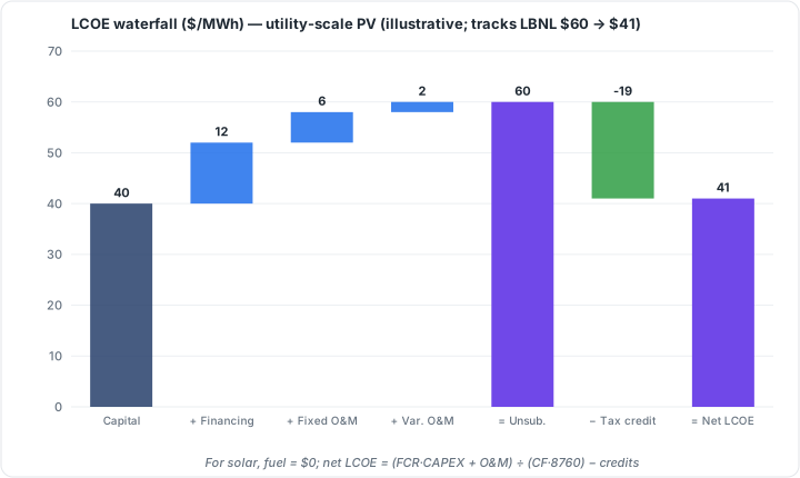 Figure 37.2: LCOE waterfall ($/MWh), utility-scale PV (illustrative; tracks LBNL $60 to $41). Original figure.
37.2 Modeling reality
A credible model includes module degradation (Ch 5.5: production declines slightly each year), utility-rate escalation (savings grow), and the incentives of Chapter 38 and net-metering/export rules of Chapter 10 (which set the value of each kWh). ⚠️ Leaving degradation or realistic derate (Ch 14/19) out of a savings projection inflates it. That is an ethics issue as much as an accuracy one (Ch 39).
37.3 Worked example: simple payback
A residential system: 8.4 kW at $2.80/W installed = $23,520. It produces 11,500 kWh/yr; the utility rate is $0.18/kWh. Assume (post-25D, cash purchase) no federal credit but a $1,000 state rebate.
- Net cost = 23,520 − 1,000 = $22,520.
- Year-1 savings = 11,500 × $0.18 = $2,070.
- Simple payback = 22,520 ÷ 2,070 ≈ 10.9 years.
- With ~3%/yr rate escalation, real payback is shorter (savings grow each year); with ~0.4%/yr degradation, slightly offsetting. A full model (Ch 19/37.2) nets these out, but the simple figure already frames the decision. ⚠️ Quote payback honestly: leaving out degradation or using an inflated production number shortens the apparent payback and burns the customer later.
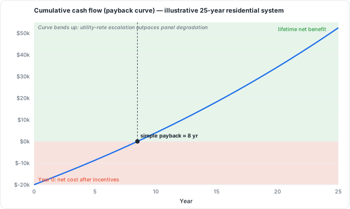 Figure 37.1: Cumulative cash flow (payback curve), illustrative residential system. Original figure.
Tools such as SAM (System Advisor Model) automate this multi-year cash-flow calculation. A performance model (weather + system specs) feeds an hourly energy output to a financial model that applies incentives, depreciation, and financing terms to produce LCOE, NPV, payback, and IRR in a single run.
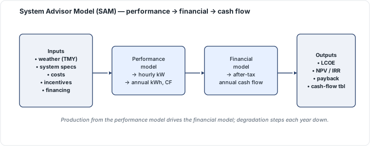 Figure 37.3: SAM model structure: performance model to financial model to cash flow. Original figure.
Chapter 37 summary
Quote installed cost in $/W; sell on payback, ROI, and (for larger buyers) LCOE/NPV. Build degradation, rate escalation, incentives, and realistic production into every projection. Overstating savings is both wrong and unethical.
- Installed cost ($/W): total system price divided by DC nameplate watts; the standard unit for comparing solar quotes.
- Payback period: net system cost divided by year-1 annual savings; the headline metric for most residential buyers.
- LCOE (Levelized Cost of Energy): lifetime project cost divided by lifetime energy output ($/kWh); the standard for utility and commercial comparisons.
- FCR (Fixed Charge Rate): annual carrying cost of capital as a fraction of total investment, derived from the CRF formula.
- WACC (Weighted-Average Cost of Capital): blended cost of debt and equity used as the discount rate in financial models.
- NPV (Net Present Value): lifetime cash flows discounted to today’s dollars; a positive value means the project earns above the cost of capital.
- Degradation: gradual annual decline in module output (typically ~0.4%/yr); must be included in honest projections.
- Rate escalation: the assumed annual rise in utility electricity prices; raises future savings and shortens real payback.
- SAM (System Advisor Model): NREL’s free tool combining performance simulation and financial modeling into a single run.
Full definitions: Appendix A (glossary).
Practice Problems: Chapter 37
- A 7 kW system costs $2.90/W installed. What’s the total price?
- It produces 9,800 kWh/yr at a $0.16/kWh rate. What are the year-1 savings?
- With no incentives, what’s the simple payback (use Q1 and Q2)?
- Why does real payback come in shorter than the simple figure when utility rates escalate?
- Name two things a dishonest proposal might omit to make payback look better, and who pays for it.
Solutions: Chapter 37
- 7,000 × $2.90 = $20,300.
- 9,800 × $0.16 = $1,568/yr.
- 20,300 ÷ 1,568 ≈ 12.9 years.
- Rising rates increase annual savings over time, so cumulative savings reach the cost sooner than a flat-rate assumption implies.
- Omitting module degradation and/or using an inflated production estimate (unrealistic derate, ignored shading); the customer pays via underdelivered savings.