18. Shading, Tilt & Azimuth Optimization

Learning objectives

• Evaluate a site’s solar access and the cost of shading.
• Choose tilt and azimuth for the project’s goal.
• Space rows to avoid self-shading and mitigate shade electronically.

18.1 The solar window and solar access

The productive hours are roughly 9 a.m.–3 p.m. solar time, when most daily energy arrives. Shading analysis quantifies obstructions across this window:

• Total Solar Resource Fraction (TSRF) / solar access %: the fraction of ideal annual irradiance a plane actually receives after shading; 100% is unshaded. Financiers and incentive programs often set minimum thresholds (e.g., 75–80%).

⚠️ Shading is non-linear: because modules series-wire, shading even part of one module can drag a whole string. Bypass diodes and MLPE mitigate this effect, but do not eliminate it.

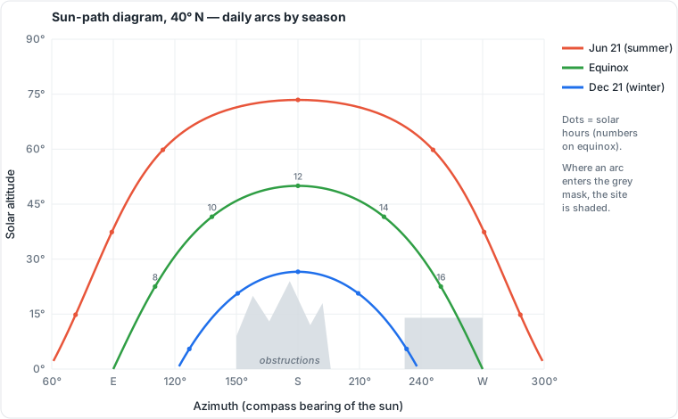Figure 18.1: Sun-path diagram, 40° N: seasonal solar arcs, with an example obstruction mask showing how a tree or building eats into the winter window. Original figure.

18.2 Tilt

• Rule of thumb: tilt ≈ site latitude for balanced annual yield.
• Latitude − 10° to 15° favors summer/annual maximum; latitude + 15° favors winter (useful for winter-peaking or off-grid worst-month sizing).
• On pitched roofs you usually accept the roof pitch; tilt optimization mainly applies to ground and flat-roof/ballasted arrays.

18.3 Azimuth

• True south (azimuth 180°, N. hemisphere) maximizes annual energy; true north in the S. hemisphere.
• East/west orientations sacrifice some annual total but shift production toward morning/evening, which is valuable under time-of-use rates or for load-matching. (Recall: true, not magnetic, south. See Chapter 2.4.)

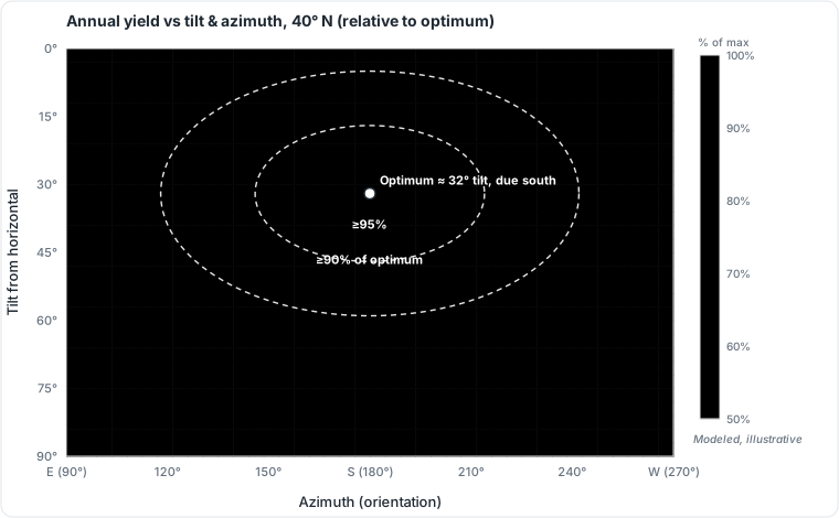Figure 18.2: Annual yield vs tilt and azimuth (40° N), relative to the optimum. Note the broad, forgiving plateau: orientation can swing well off south and tilt off ideal with only single-digit losses. Modeled, original figure.

18.4 Inter-row spacing

For ground mounts and flat-roof tilted arrays, rows must be spaced so a front row doesn’t shade the one behind during the solar window. The required pitch is a function of latitude, tilt, and the winter sun angle. Tighter spacing fits more kW but costs energy to self-shading; the ground coverage ratio (GCR) captures this trade.

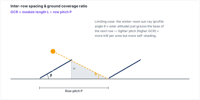Figure 18.3: Inter-row spacing and the ground coverage ratio (GCR = module length L ÷ row pitch P). The limiting case sizes the pitch so the winter-noon ray just grazes the next row. Original figure.

18.5 Tools and mitigation

Shade is measured with tools like the Solar Pathfinder, drone/photo-based apps, or design software (Aurora, HelioScope) that compute TSRF and model losses. Where shade is unavoidable, MLPE (microinverters/optimizers, Chapter 6.2) limits its spread by isolating affected modules.

18.6 Worked example: the series-shading penalty

A string of 10 modules produces 4,000 W in full sun. A chimney shades one module so its bypass diode activates, removing roughly that module’s contribution and disrupting the string’s operating point. Without module-level electronics, the string can drop far more than the naive 1/10 (10%): often 20–30%+ depending on conditions, because the shaded cell drags the whole series circuit. Add microinverters or optimizers (MLPE) and the loss is largely confined to the one affected module (~10%). ⚠️ This nonlinearity is why a single tree branch or vent pipe matters so much. Shade analysis (TSRF) must precede any quote.

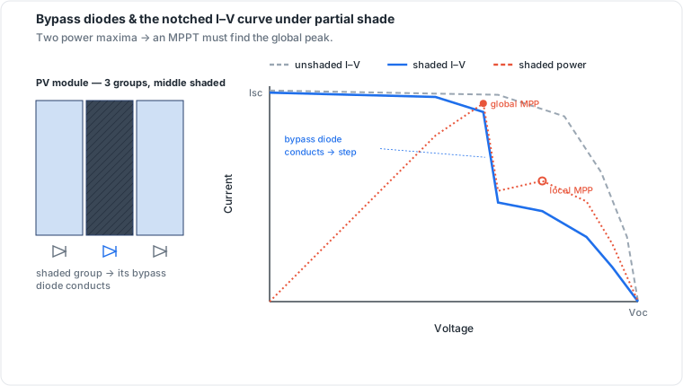Figure 18.4: Bypass diodes and the notched I–V curve under partial shade. The bypass diode reroutes current around the shaded group, leaving a step in the I–V curve and two power maxima. This is why an MPPT must search for the global peak. Original figure.

Tilt/azimuth quick reference:

• Annual max: face true south (N. hemisphere), tilt ≈ latitude.
• Summer bias: tilt ≈ latitude − 15°. Winter bias: tilt ≈ latitude + 15°.
• TOU rate optimization: shift toward west to push production into expensive late-afternoon hours.

Chapter 18 summary

Assess solar access (TSRF) across the 9–3 window; shading hurts disproportionately because of series wiring. Set tilt near latitude (±15° to bias seasons) and azimuth to true south for annual max or east/west for TOU. Space rows by GCR to avoid self-shading. Measure with shade tools and mitigate residual shade with MLPE.

Practice Problems: Chapter 18

1. A roof plane has a TSRF of 78%. What does that number mean?
2. Why can shading one module in a 12-module series string cost much more than 1/12 of the string’s output?
3. A site is at 40° latitude. What fixed tilt gives balanced annual yield, and what tilt would you choose to favor winter production?
4. A homeowner is on a time-of-use rate that pays most at 4–8 PM. Their south roof is full; an east and a west plane remain. Which should you prefer for the next array, and why?
5. What design measure most directly limits the spread of a shading loss across a string?
6. On a ground mount, what happens if rows are spaced too tightly, and what ratio captures the trade-off?

Solutions: Chapter 18

1. The plane receives 78% of the irradiance an ideal unshaded plane would over the year (22% lost to shading/orientation).
2. Series wiring makes one shaded module a bottleneck that drags the whole string’s operating point; the bypass diode reroutes around it but the string still loses more than the single module’s share.
3. Balanced: tilt ≈ 40°. Winter bias: tilt ≈ 55° (latitude + 15°).
4. The west plane: it shifts production into the 4–8 PM high-value window, maximizing bill savings under that TOU rate even if annual kWh is slightly lower.
5. Module-level power electronics (MLPE): microinverters or optimizers isolate each module.
6. Front rows self-shade the rows behind during low winter sun, costing energy; the ground coverage ratio (GCR) captures the packing-vs-shading trade-off.