13. Load Analysis & Energy Audits
Learning objectives
- Start every design from demand, not panel count.
- Extract the right numbers from a utility bill.
- Distinguish energy (kWh) sizing from power (kW) concerns.
- Apply the efficiency-first principle before sizing generation.
13.1 Demand comes first
Amateurs start with “how many panels fit?” Professionals start with “how much energy does this site need, and when?” Every kW of array is justified by a kWh of demand. The deliverable of this chapter is a defensible annual energy target (and, for off-grid, a daily one).
13.2 Reading the utility bill
For a grid-tied residential job, the customer’s bills are the primary data:
- Annual consumption (kWh/yr): sum twelve months; this is the headline number you’ll size against.
- Monthly profile: the shape across the year reveals summer A/C or winter heating peaks that affect seasonal design and storage value.
- Rate structure: flat, tiered, or time-of-use; and the export rule (net metering vs net billing, Chapter 10).
TOU + poor export economics push toward storage and self-consumption.
Example 13.A: A home’s twelve bills sum to 11,400 kWh/yr, averaging ~950 kWh/month, peaking in summer. If the customer wants to offset 100% of usage, the array energy target is 11,400 kWh/yr, which becomes the input to Chapter 14.
13.3 The off-grid load inventory
Off-grid (Chapter 11) has no bill to read, so you build demand bottom-up: list every load, its power draw (W), and hours of daily use, to get watt-hours per day. This inventory is unforgiving: a missed well-pump or an optimistic refrigerator estimate propagates into an undersized battery bank.
Example 13.B: Lights 5 × 10 W × 5 h = 250 Wh; fridge 150 W × 8 h (compressor duty) = 1,200 Wh; laptop 60 W × 4 h = 240 Wh; pump 800 W × 1 h = 800 Wh → partial daily total ≈ 2,490 Wh/day, before adding the rest and a safety margin.
13.4 Efficiency first
The cheapest kWh is the one you never need to generate. Before sizing, identify efficiency wins (LED lighting, heat-pump upgrades, phantom-load elimination) because every watt-hour trimmed shrinks array, inverter, and (off-grid) battery cost simultaneously. This is doubly true off-grid, where generation/storage is expensive.
13.5 Worked example: an off-grid load table
Bottom-up load inventories are best built as a table. For a small cabin:
| Load | Power (W) | Hours/day | Wh/day |
|---|---|---|---|
| LED lights (×6) | 60 total | 5 | 300 |
| Refrigerator (compressor duty) | 150 | 8 | 1,200 |
| Water pump | 800 | 1 | 800 |
| Laptop + router | 90 | 5 | 450 |
| Phone/misc charging | 40 | 3 | 120 |
| Subtotal | 2,870 | ||
| Safety margin (+25%) | +718 | ||
| Design daily load | ≈ 3,590 Wh/day |
⚠️ The margin isn’t padding for its own sake: it covers forgotten loads, cloudy-day behavior, and future creep. The 3,590 Wh/day figure now drives both array sizing (Ch 14) and battery sizing (Ch 17).
13.6 Load-profile shape and the duck curve
A bill’s annual kWh total tells you how much to generate; the daily load-profile shape tells you when demand arrives, which is what storage and rate-structure decisions turn on.
Residential daily profile. Load tracks household routines. Demand is lowest overnight, bottoming around 5:00 a.m. (only always-on baseload devices: refrigerators, networking equipment, standby power). It climbs through the morning and peaks in a season-dependent pattern:
- Summer: a single broad peak around 5–6 p.m., driven by air conditioning (present in 87% of U.S. homes). The U.S. annual grid peak falls in summer for this reason.
- Winter: a twin-peak shape, with a morning spike (lighting, heating, hot water, businesses opening) and an evening spike (people home, heating, cooking), separated by a mid-afternoon lull.
- Spring/autumn: lowest overall load, with little heating or cooling demand.
Weekends and holidays run noticeably lower than weekdays. Utility on-peak windows (typically 7 a.m.–11 p.m. weekdays) reflect this weekday/weekend split.
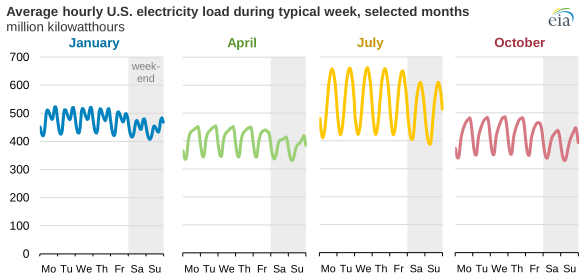
Figure 13.1: Average hourly U.S. load, typical week. Source: EIA Today in Energy (public domain).
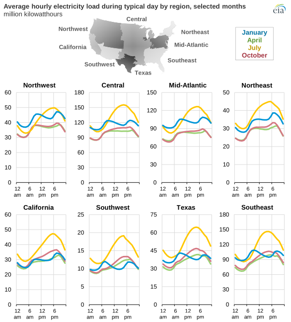
Figure 13.2: Average hourly load by U.S. region. Source: EIA Today in Energy (public domain).
Why this matters for PV. Solar generation peaks at midday and drops to zero by early evening, yet residential demand peaks at 5–6 p.m. in summer. That mismatch is the core problem load analysis exists to expose: the array produces when nobody is home; the load spikes after the sun sets. Storage or load-shifting (dishwashers, EV charging, pool pumps scheduled to midday) bridges the gap.
The duck curve. When enough rooftop and utility-scale solar is on the grid, the net load (demand minus variable renewable generation) develops a distinctive shape. Midday solar carves a belly out of net load, and as the sun sets while demand stays high, net load ramps steeply upward into the evening, tracing the profile of a duck’s neck. The steeper the ramp, the harder it is for dispatchable plants (gas peakers, storage) to respond fast enough.
The CAISO grid in California, with high solar penetration, shows this clearly: on high-solar days the evening net-load ramp exceeds 11,000 MW within three hours (13,000 MW in spring). California’s midday dip has deepened every year as solar capacity grows. That trend has driven a parallel buildout of grid-scale battery storage, from 0.2 GW in 2018 to 4.9 GW by April 2023. The storage chapters (Ch 17, 18) address how a behind-the-meter battery can flatten the belly (charging midday) and shorten the neck (discharging in the evening peak).
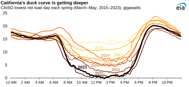
Figure 13.3: California’s duck curve is getting deeper, 2018–2023. Source: EIA Today in Energy (public domain).
Chapter 13 summary
Size from demand. Grid-tied: pull annual kWh, the monthly profile, and the rate/export structure off the bills. Off-grid: build a bottom-up Wh/day load inventory. Apply efficiency improvements first, since they shrink every downstream component. Output: an annual (or daily) energy target.
- Annual energy target: the total kWh/yr (or Wh/day off-grid) a system must produce; the primary output of load analysis and the input to array sizing.
- Load profile: a time-of-day plot of electricity demand showing when a site uses power and how much; drives storage sizing and rate-structure decisions.
- TOU (Time-of-Use) rate: a utility pricing structure with higher rates during on-peak hours and lower rates off-peak; increases the value of self-consumption and storage.
- Duck curve: the net-load shape that develops when high solar penetration carves a midday belly out of grid demand, followed by a steep evening ramp as generation drops and load peaks.
- Net load: total electricity demand minus variable renewable generation; the quantity grid operators must dispatch from controllable sources.
- Wh/day (watt-hours per day): the off-grid energy unit used in load inventories; power (W) multiplied by hours of use per day.
- Safety margin: a 25% (or similar) buffer added to the design daily load to cover forgotten loads, cloudy-day behavior, and future growth.
Full definitions: Appendix A (glossary).
Practice Problems: Chapter 13
- A homeowner’s 12 monthly bills total 13,800 kWh. What is the annual energy target to offset 100% of use?
- The same home averages how many kWh per month?
- An off-grid load table sums to 4,200 Wh/day. Adding a 25% safety margin, what is the design daily load?
- Why does an efficiency upgrade (e.g., swapping an old fridge) reduce three downstream component costs off-grid, not one?
- A bill shows summer usage triple the winter usage. What does that pattern most likely indicate, and why does it matter for design?
Solutions: Chapter 13
- 13,800 kWh/yr (the sum is the target for a full offset).
- 13,800 ÷ 12 = 1,150 kWh/month.
- 4,200 × 1.25 = 5,250 Wh/day.
- Less daily energy means a smaller array, a smaller battery bank, and a smaller inverter/charge controller. All three scale with the load off-grid, so trimming demand shrinks each.
- Heavy summer air-conditioning load; it matters because it shifts the production target toward summer and affects whether storage/TOU strategies pay off (Ch 12, 18).